Tracing Particles between Snapshots

The bridge module has tools for connecting different outputs which allows you to trace particles from one snapshot of the simulation to another.

In pynbody, a Bridge is an object that links two snapshots together. Once connected, a bridge object called on a specific subset of particles in one snapshot will trace these particles back (or forward) to the second snapshot. Constructing bridges is also very straight-forward in most cases.

Since the pynbody test data does not include a simulation with two different outputs, we will borrow some test data from tangos to illustrate the point. Click here to download, or type

$ wget https://zenodo.org/records/10825178/files/tutorial_gadget4.tar.gz?download=1 -O tutorial_gadget4.tar.gz
$ tar -xvzf tutorial_gadget4.tar.gz

Basic usage

Load the data at high and low redshift:

In [1]: import pynbody

In [2]: f1 = pynbody.load("tutorial_gadget4/snapshot_033.hdf5")

In [3]: f2 = pynbody.load("tutorial_gadget4/snapshot_035.hdf5")

Verify the redshifts:

In [4]: f"f1 redshift={f1.properties['z']:.2f}; f2 redshift={f2.properties['z']:.2f}"
Out[4]: 'f1 redshift=1.35; f2 redshift=1.06'

Load the halo catalogue at low redshift:

In [5]: h2 = f2.halos()

Create the bridge object:

In [6]: b = f2.bridge(f1)

b is now an Bridge object that links the two outputs f1 and f2 together. Note that you can either bridge from f2 to f1 (as here) or from f1 to ``f2``and it makes no difference at all to basic functionality: the bridge can be traversed in either direction.

Note

There are different subclasses of bridge that implement the mapping back and forth in different ways, and by default the:func:~pynbody.snapshot.SimSnap.bridge method will attempt to choose the best possible option, by inspecting the file formats. However, if you prefer, you can explicitly instantiate the bridge for yourself (see below).

Passing a SubSnap from one of the two linked snapshots to b will return a SubSnap with the same particles in the other snapshot. To take a really simple example, we might want to calculate the typical comoving distance travelled by particles between the two snapshots. Without a bridge, this is hard; specifically, note that the following gives the wrong answer:

In [7]: displacement = np.linalg.norm(f2['pos'] - f1['pos'], axis=1).in_units("Mpc") # <-- wrong thing to do

In [8]: displacement.mean() # <-- will give wrong answer
Out[8]: SimArray(2.6222446, dtype=float32, 'Mpc')

This seems like a very long way for a particle to have travelled on average between two quite closely spaced snapshots — because it’s wrong. Gadbget has re-ordered the particles between the two snapshots, the particle with index 0 in the first snapshot is not the same particle as the one with index 0 in the second snapshot. So the above answer involves randomly shuffling particles. What we actually wanted to do was to trace the particles from one snapshot to the other, and then calculate the distance travelled by each particle. This is what the bridge does:

In [9]: f2_particles_reordered = b(f1)

In [10]: displacement = np.linalg.norm(f2_particles_reordered['pos'] - f1['pos'], axis=1).in_units("Mpc")

In [11]: displacement.mean()
Out[11]: SimArray(0.39596593, dtype=float32, 'Mpc')

This is the correct (and much more reasonable) answer.

Tracing subregions

Bridges are not just about correcting the order of particles for comparisons like this; we can also select subsets of the full snapshot. If we want to see where all the particles that are in halo 9 in the low-redshift snapshot (f1) came from at low redshift (f2), we can simply do:

In [12]: progenitor_particles = b(h2[9])

progenitor_particles now contains the particles in snapshot 1 that will later collapse into halo 9 in snapshot 2. To verify, we can explicitly check that pynbody has selected out the correct particles according to their unique identifier (iord):

In [13]: h2[9]['iord']
Out[13]: 
SimArray([3753184, 3796702, 3752676, ..., 3358768, 3401255, 4101555],
         dtype=uint32)

In [14]: progenitor_particles['iord']
Out[14]: 
SimArray([3753184, 3796702, 3752676, ..., 3358768, 3401255, 4101555],
         dtype=uint32)

In [15]: all(h2[9]['iord'] == progenitor_particles['iord'])
Out[15]: True

But of course the actual particle properties are different in the two cases, being taken from the two snapshots, e.g.

In [16]: progenitor_particles['x']
Out[16]: 
SimArray([24.372095, 24.371895, 24.37157 , ..., 24.266537, 24.269943,
          24.413738], dtype=float32, '3.09e+24 cm a h**-1')

In [17]: h2[9]['x']
Out[17]: 
SimArray([24.320396, 24.320671, 24.32054 , ..., 24.284363, 24.290815,
          24.306082], dtype=float32, '3.09e+24 cm a h**-1')

We can now make a plot to see where the particles in halo 8 at low redshift were in the higher redshift snapshot:

In [18]: import matplotlib.pyplot as p

In [19]: p.plot(h2[7]['x'], h2[7]['y'], 'b.', label=f"z={f2.properties['z']:.2f} halo 7")
Out[19]: [<matplotlib.lines.Line2D at 0x7f19926e89d0>]

In [20]: p.plot(b(h2[7])['x'], b(h2[7])['y'], 'r.', label=f"Tracked to z={f1.properties['z']:.2f}")
Out[20]: [<matplotlib.lines.Line2D at 0x7f1991d6cfd0>]

In [21]: p.ylim(27.25, 27.75); p.xlim(24.6, 25.2); p.gca().set_aspect('equal')

In [22]: p.legend()
Out[22]: <matplotlib.legend.Legend at 0x7f1991c85410>

In [23]: p.xlabel('x / code units'); p.ylabel('y / code units')
Out[23]: Text(0, 0.5, 'y / code units')

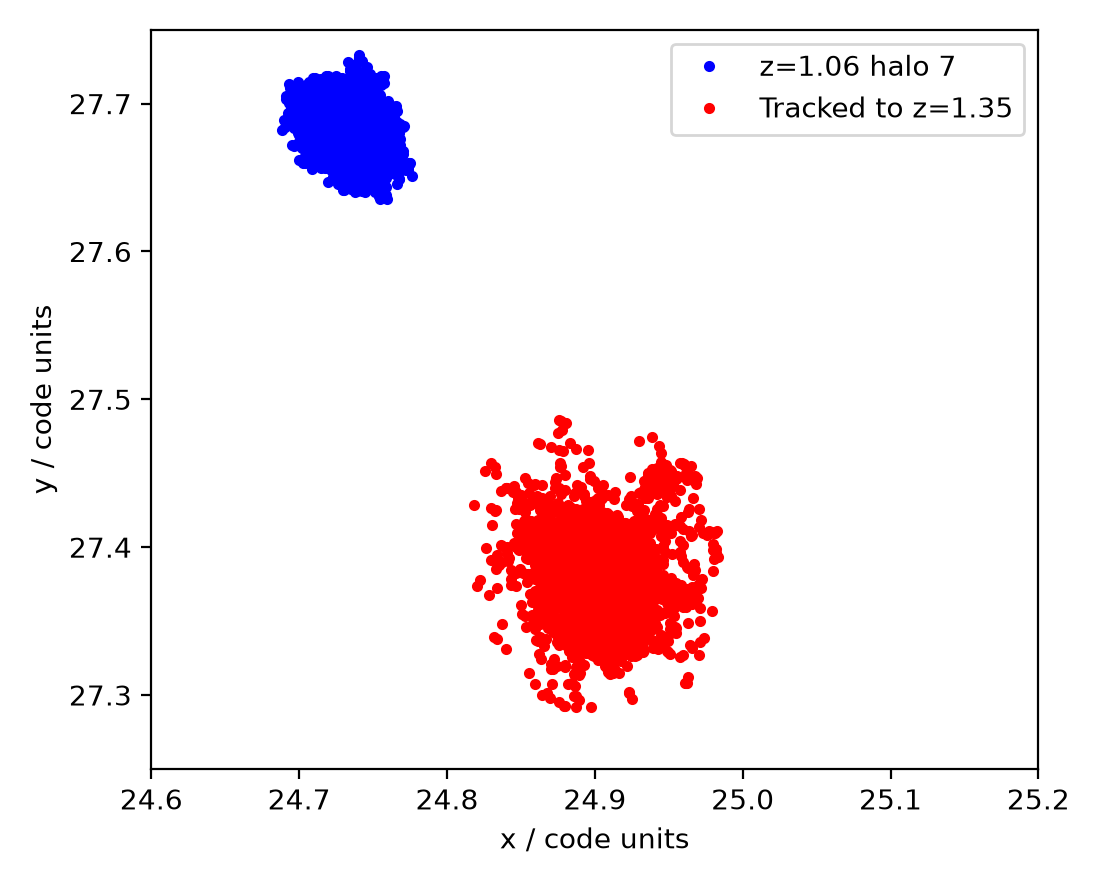
From this we can see that the particles in halo 7 at z=1.06 (blue) are more compact than the same particles at z=1.35 (red), and that the comoving position of the halo centre has also drifted as expected from the earlier calculations.

Identifying halos between different outputs

Changed in version 2.0: Interface for halo matching

The methods match_halos(), fuzzy_match_halos() and an underlying method count_particles_in_common() were added in version 2.0, and should be preferred to older methods (match_catalog(), fuzzy_match_catalog()). The latter provide similar functionality but with an inconsistent interface; they are now deprecated and should not be used in new code.

You may wish to work out how a halo catalogue maps onto a halo catalogue for a different output. Just as with particles, the ordering of halos can be expected to change between snapshots, so if we get a halo catalogue for the earlier snapshot, we’ll find halo 7 is not the same as halo 7 in the later snapshot:

In [24]: h1 = f1.halos()

In [25]: h1[7]['pos'].mean(axis=0)
Out[25]: SimArray([22.933945, 27.054394, 25.959143], dtype=float32, '3.09e+24 cm a h**-1')

In [26]: b(h2[7])['pos'].mean(axis=0)
Out[26]: SimArray([24.903126, 27.381052, 24.72228 ], dtype=float32, '3.09e+24 cm a h**-1')

A glance at the positions of these rough halo centres show they can’t be the same set of particles.

To map correctly between halo catalogues at different redshifts, we can use match_halos():

In [27]: matching = b.match_halos(h2, h1)

In [28]: matching[7]
Out[28]: 8

Here, matching is a dictionary that maps from halo numbers in h2 (the low redshift snapshot) to halo numbers in h1 (the high redshift snapshot). The above code is telling us that halo 7 in the low-redshift snapshot is the same as halo 8 in the high-redshift snapshot. Let’s test that graphically:

In [29]: p.plot(h1[8]['x'], h1[8]['y'], 'k.', label=f"z={f1.properties['z']:.2f} halo 8")
Out[29]: [<matplotlib.lines.Line2D at 0x7f198840a890>]

In [30]: p.legend()
Out[30]: <matplotlib.legend.Legend at 0x7f1991cc66d0>

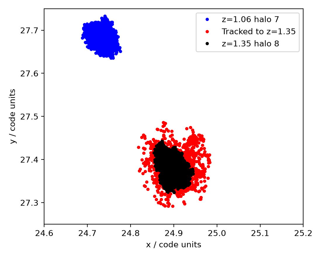
As expected, the particles that make up halo 8 (black) in the high-redshift snapshot are almost coincident with those that we tracked from halo 7 in the low-redshift snapshot (red). Some of the tracked halo 7 particles haven’t yet accreted, so it’s smaller, but the centres are almost coincident.

We can also see if there were any mergers or transfer between different structures by calling fuzzy_match_halos():

In [31]: fuzzy_matching = b.fuzzy_match_halos(h2, h1)

In [32]: fuzzy_matching[7]
Out[32]: [(8, 0.9741290100034494), (770, 0.018454639530872716)]

This tells us that as well as halo 8, which contributed most of the particles, about 1.8% of the particles were contributed by halo 770. Let’s plot that too, for good measure:

In [33]: p.plot(h1[770]['x'], h1[770]['y'], 'y.', label=f"z={f1.properties['z']:.2f} halo 770")
Out[33]: [<matplotlib.lines.Line2D at 0x7f1988322890>]

In [34]: p.legend()
Out[34]: <matplotlib.legend.Legend at 0x7f198831e6d0>

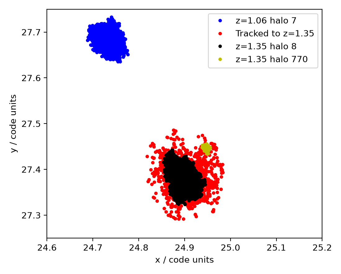
It shows up in yellow and, as expected, it looks like it’s falling in.

Note

Some halo finders generate a merger tree that can provide some of this information, in which case it is available through the properties of the halo catalogues themselves. (See Halos in Pynbody for more information on halo properties.) However, the bridge is a more general tool that can be used to trace any subset of particles between two snapshots, not just those that are part of a halo catalogue, and furthermore can be applied to snapshots which are not necessarily adjacent in time. It can also be used to match halos between different simulations, e.g. DMO and hydro runs.

There can be an overwhelming amount of information returned by the bridge. To digest cosmological information, we recommend the use of pynbody’s sister package, tangos.

Which class to use?

There is a built-in-logic which selects the best possible subclass of Bridge when you call the method bridge(). However, you can equally well choose the bridge and its options for yourself, and sometimes bridge() will tell you it can’t decide what kind of bridge to generate.

For files where the particle ordering is static, so that the particle with index i in the first snapshot also has index i in the second snapshot, use the Bridge class, as follows:

b = pynbody.bridge.Bridge(f1, f2)

For files which can spawn new particles, and therefore have a monotonically increasing particle ordering array (e.g. “iord” in gasoline), use the OrderBridge class:

b = pynbody.bridge.OrderBridge(f1, f2)

Snapshot formats where the particle ordering can change require a more processor and memory intensive mapping algorithm to be used, which you can enable by asking for it explicitly:

b = pynbody.bridge.OrderBridge(f1, f2, monotonic=False)