Halo Mass function

This recipe makes use of the module halo to generate the halo mass function of a given snapshot and compare it to a theoretical model.

Note

The halo mass function code in pynbody was implemented in 2012 when there were no other python libraries that could calculate theoretical HMFs. Since then, cosmology-focussed libraries such as hmf, Colossus and CCL have been developed. For precision cosmology applications, we recommend using these libraries. The functionality here is retained for quick cross-checks of simulations.

Since the pynbody test data does not include a simulation with a uniform resolution volume, we will borrow some test data from tangos to illustrate the halo mass function. Click here to download, or type

$ wget https://zenodo.org/records/10825178/files/tutorial_gadget.tar.gz?download=1 -O tutorial_gadget4.tar.gz
$ tar -xvzf tutorial_gadget.tar.gz

Calculating a theoretical halo mass function

We will start by loading a snapshot data.

In [1]: import pynbody
   ...: import matplotlib.pyplot as p
   ...: s = pynbody.load('tutorial_gadget/snapshot_020')
   ...: s.physical_units()
   ...: 

To define the expected halo mass function, we need to make sure that the cosmology is well set. Some cosmological parameters are carried by the snapshot itself. However, others like sigma_8 are usually not, so you might want to specify it to the value used to create the simulation. In this particular file, we can check the density and Hubble parameters then set sigma8.

In [2]: s.properties['omegaM0'], s.properties['omegaL0'], s.properties['h']
Out[2]: (0.279, 0.721, 0.701)

In [3]: s.properties['sigma8'] = 0.8288

You can generate an HMF using the halo_mass_function() function as follows.

In [4]: m, sig, dn_dlogm = pynbody.analysis.hmf.halo_mass_function(s, log_M_min=10, log_M_max=15, delta_log_M=0.1,
   ...:                                                            kern="REEDU")
   ...: 

By specifying kern="REEDU", we are asking for a Reed (2007) mass function. Other options are described in the documentation of halo_mass_function().

Let’s inspect the output:

In [5]: p.plot(m, dn_dlogm)
Out[5]: [<matplotlib.lines.Line2D at 0x7f1991d52f10>]

In [6]: p.loglog()
Out[6]: []

In [7]: p.xlabel(f"$M / {m.units.latex()}$")
Out[7]: Text(0.5, 0, '$M / M_{\\odot}\\,\\mathrm{h}^{-1}$')

In [8]: p.ylabel(f"$dn / d\\log M / {dn_dlogm.units.latex()}$")
Out[8]: Text(0, 0.5, '$dn / d\\log M / \\mathrm{Mpc}^{-3}\\,\\mathrm{h}^{3}\\,\\mathrm{a}^{-3}$')

Obtaining the binned halo mass function from the simulation

We now generate the HMF from binned halo counts in a simulation volume.

This method calculates all halo masses contained in the snapshot and bin them in a given mass range. The number count is then normalised by the simulation volume to obtain the snapshot HMF. We can get a sense of error bars from the number count in each bin assuming a Poissonian distribution:

In [9]: bin_center, bin_counts, err = pynbody.analysis.hmf.simulation_halo_mass_function(s,
   ...:                        log_M_min=10, log_M_max=15, delta_log_M=0.1, )
   ...: 

We are now ready to compare the two results on a plot:

In [10]: plt.errorbar(bin_center, bin_counts, yerr=err, fmt='o',
   ....:              capthick=2, elinewidth=2, color='darkgoldenrod')
   ....: 
Out[10]: <ErrorbarContainer object of 3 artists>

In [11]: plt.xlim(1e10, 1e15)
Out[11]: (10000000000.0, 1000000000000000.0)

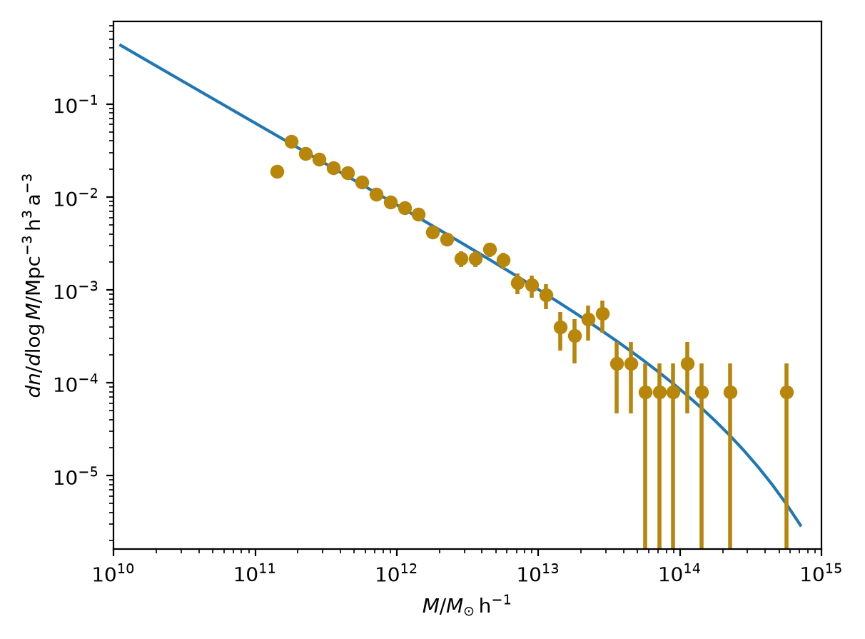
The agreement is pretty good. Note that in generating the empirical halo mass function above, Pynbody has summed the mass of particles in each halo to get the halo mass. This may not be what you want, especially e.g. if you want to compare with virial masses rather than bound masses. Furthermore, summing over particles for each halo can be slow for large simulations. For all these reasons, if the halo finder provides pre-calculated masses you can use those instead by passing them to the mass_property argument of simulation_halo_mass_function(). First, check the available properties for your halo catalogue:

In [12]: s.halos()[0].properties.keys()
Out[12]: dict_keys(['omegaM0', 'omegaL0', 'boxsize', 'a', 'h', 'time', 'sigma8', 'halo_number', 'mass', 'pos', 'mmean_200', 'rmean_200', 'mcrit_200', 'rcrit_200', 'mtop_200', 'rtop_200', 'contmass', 'group_len', 'group_off', 'first_sub', 'Nsubs', 'cont_count', 'mostboundID', 'children'])

Here we can see SubFind calculated various mass definitions like mmean_200, mcrit_200 etc. The particular properties available will depend on your halo finder. Let’s use mmean_200 as another comparison with the HMF:

In [13]: bin_center, bin_counts, err = pynbody.analysis.hmf.simulation_halo_mass_function(s,
   ....:                        log_M_min=10, log_M_max=15, delta_log_M=0.1,
   ....:                        mass_property='mmean_200')
   ....: 

In [14]: plt.errorbar(bin_center, bin_counts, yerr=err, fmt='o',
   ....:              capthick=2, elinewidth=2, color='k', alpha=0.5)
   ....: 
Out[14]: <ErrorbarContainer object of 3 artists>

In [15]: plt.xlim(1e10, 1e15)
Out[15]: (10000000000.0, 1000000000000000.0)

You can see that this agrees well. The slight change is expected because of the change in halo mass definition from a FoF mass to a spherical overdensity mass. The disagreement at low masses is due to the finite resolution of the simulation.