Images#
This tutorial walks you through a number of pynbody’s image-making features. If you have not yet done so, it is advisable to work through the quick-start tutorial first, for a broader introduction.
Note
To illustrate pynbody’s image-generation to best effect, here we make use of a snapshot from a
high-resolution zoom simulation that is not actually part of pynbody’s test data suite (since it
is >10 GB in size). If you want to try out these image-making operations for yourself, you can
easily substitute your own simulation or a galaxy from the test suite, e.g. testdata/gasoline_ahf/g15784.lr.01024).
This tutorial is generated from a ipython notebook which you can access directly using the download link at the top right. We’ll start by setting up matplotlib and loading our file and halo catalogue:
In [2]:
import pynbody

f = pynbody.load("halo685_tng/snapdir_261/snap_261")
# Note, replace the above filename with testdata/gasoline_ahf/g15784.lr.01024 if you want to use
# the pynbody test data.

h = f.halos()
f.physical_units()

pynbody.analysis.center(h[0])
/Users/app/Science/pynbody/pynbody/snapshot/gadgethdf.py:403: UserWarning: Masses are either stored in the header or have another dataset name; assuming the cosmological factor h**-1
  warnings.warn("Masses are either stored in the header or have another dataset name; assuming the cosmological factor %s" % units.h**-1)
Out[2]:
<Transformation translate, offset_velocity>
Now we make the first plot, similar to the one made in the quick-start tutorial. We will
ask for a projected density plot, simply by telling pynbody that we would like units of Msol kpc^-2.
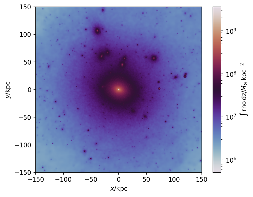
First, we will look at the dark matter distribution in the halo. The width of the image is set to 300 kpc.
In [3]:
pynbody.plot.image(f.dm, width="300 kpc", units="Msol kpc^-2", cmap="twilight")
Pynbody is aware of the periodicity of cosmological simulations, so if you make a zoomed-out image, you will see structures repeating. Here, we set the image width to 100 Mpc, but the box size is only around 70 Mpc, so the periodicity in the large scale structure starts to become visible.
In [4]:
pynbody.plot.image(f.dm, width="100 Mpc", units="Msol kpc^-2", cmap="twilight")

We can switch to estimating density of other particles just by passing in the appropriate family view of the simulation. Switching from f.dm to f.gas lets use see the central galaxy’s gas content.
In [5]:
pynbody.plot.image(f.gas, width="100 kpc", units="Msol kpc^-2", cmap="bone")

Next, we transform the simulation to look at the disk face-on. Note that the surface density is always with respect to the line of sight, so once transformed we are getting the true gas surface density of the disk.
In [6]:
with pynbody.analysis.faceon(h[0]):
    pynbody.plot.image(f.gas, width="100 kpc", units="Msol kpc^-2", cmap="bone",
                       colorbar_label=r"$\Sigma_{\mathrm{gas}} / M_{\odot}\,\mathrm{kpc}^{-2}$")

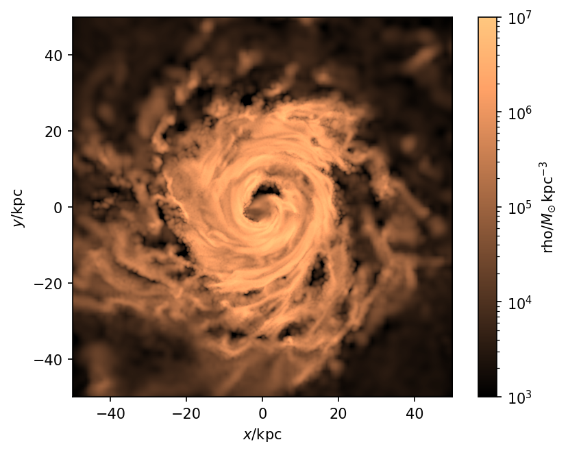
Next, we are going to switch to looking at the physical (unprojected) density. We can do this simply by removing the units keyword, to get a view of the density in a thin plane through z=0. This is the disk plane if we continue to wrap the image command inside the faceon context. We also provide an explicit vmin and vmax to give the minimum and maximum values in the colormap. In the previous examples, the default was used, in which the colormap is scaled to the minimum and maximum
values in the image. However the dynamic range of the density is too large for that, so we specify our own min/max.
In [7]:
with pynbody.analysis.faceon(h[0]):
    pynbody.plot.image(f.gas, width="100 kpc", cmap="copper", vmin=1e3, vmax=1e7)
Plotting other quantities#
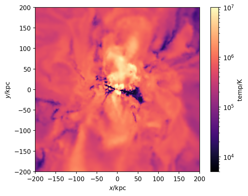
So far, we have been plotting the density, but we can specify any other quantity via the second argument of image. We can pass either an array (which must match the length of the snapshot being imaged), or the name of an array within the snapshot. Here we ask for the temperature. Note the width has been increased to 400 kpc, so we are looking at the temperature structure of the circumgalactic medium. Just as by default the density plot would return a slice through the z=0 plane, so here too
we get the temperature in a thin slice through z=0.
In [8]:
pynbody.plot.image(f.gas, 'temp', width="400 kpc", cmap="magma", vmin=0.5e4, vmax=1e7)

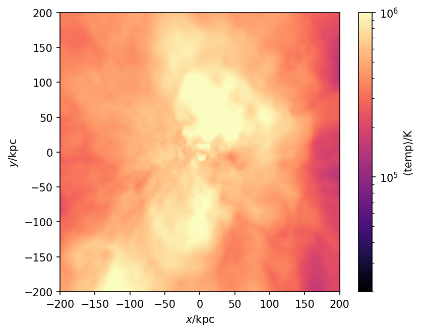
The image looks good, but a little grainy. The graininess is due to SPH interpolation being inherently noisy. To smoothly interpolate temperature values rather than make strict SPH estimates, pass denoise=True. This looks better:
In [9]:
pynbody.plot.image(f.gas, qty='temp', width="400 kpc", cmap="magma", vmin=0.5e4, vmax=1e7, denoise=True)
Just as we can project the density, we can also project other quantities. However for this we need to be a bit more specific about what we want, and weight it down the z-axis (line of sight) with respect to another variable. This variable is passed in the weight keyword. For example, a density-weighted temperature map is obtained as follows:
In [10]:
pynbody.plot.image(f.gas, qty='temp', width="400 kpc", cmap="magma", vmin=2e4,vmax=1e6,
                   weight='rho')

Due to the density-weighting, the temperature map in the centre is dominated by the disk. This may be exactly the appropriate view, but in other cases you might prefer a volume-weighted average. This is obtained by passing weight=True. Note, however, that this can cause the result to be dominated by the entire intergalactic medium through which the line of sight passes. Therefore we restrict the z-range to the same as the image width, by passing restrict_depth=True. Since our width is
400 kpc, this implies \(-200 < z < 200\) kpc. This looks very different:
In [11]:
pynbody.plot.image(f.gas, qty='temp', width="400 kpc", cmap="magma", vmin=2e4,vmax=1e6,
                   weight=True, restrict_depth=True)
Velocity images#
One often wants to understand the flow of gas as well as its thermodynamic properties. Pynbody can overplot velocity information on top of an image. Here we plot the temperature, but overlay the velocity field as a quiver plot. There are a lot of options controlling the appearance of the velocity field; perhaps most importantly, the vector_scale keyword controls the length of the arrows by specifying how large the velocity would need to be for the arrow to occupy the full plot width. The
key_length keyword, on the other hand, specifies the length of the arrow to show in the key.
In [12]:
pynbody.plot.sph.velocity_image(f.gas, qty='temp', width="400 kpc", cmap="magma",
                                vmin=2e4, vmax=1e6,
                                vector_scale="1e4 km s^-1", key_length = "1000 km s^-1",
                                key_bg_color='white')

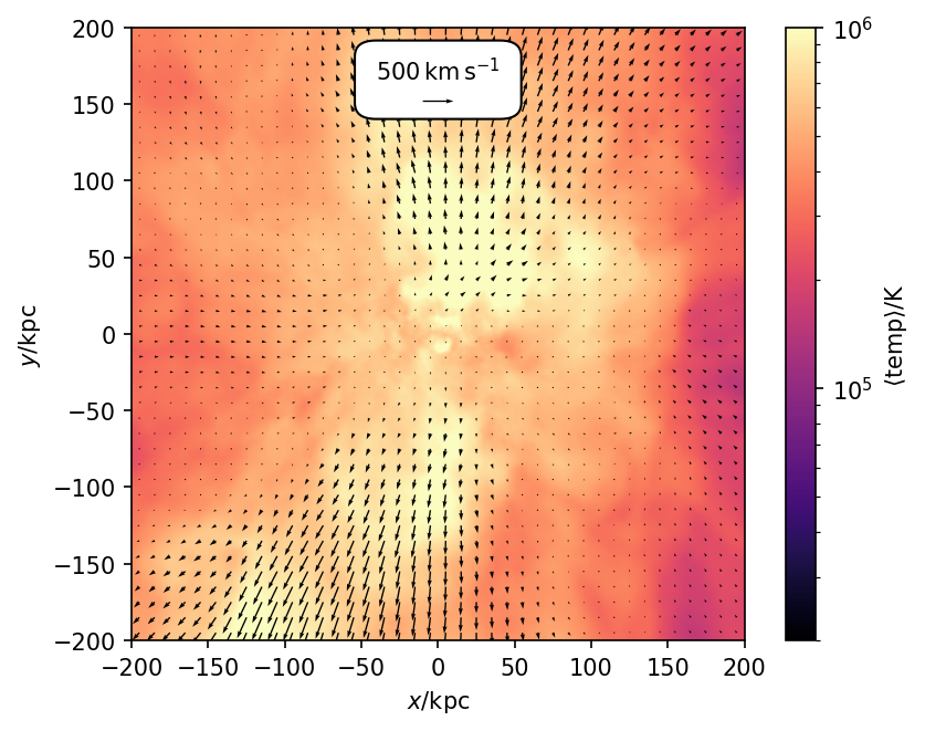
One may combine velocity imaging with averaging along the line of sight. Here we return to the volume-weighted temperature map, but overlay the velocity field. The velocity field is weighted and restricted in depth in just the same way as the underlying map:
In [13]:
pynbody.plot.sph.velocity_image(f.gas, qty='temp', width="400 kpc", cmap="magma",
                                vmin=2e4, vmax=1e6,
                                vector_scale="1e4 km s^-1", key_length = "500 km s^-1",
                                weight=True, restrict_depth=True)
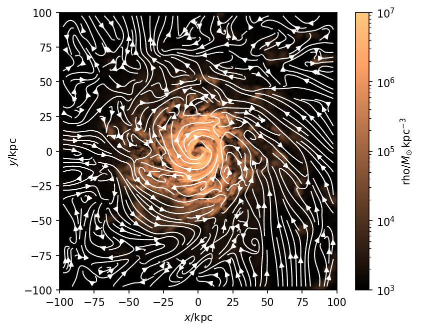
For some purposes, streamplots are better than quiver fields. These can be enabled by setting mode='stream'. Here, we make a face-on slice of the density, and the corresponding slice of the velocity field is used to make streamlines. Note also that we can set vector_color='white' to make the streamlines more visible on this particular background.
In [14]:
with pynbody.analysis.faceon(h[0]):
    pynbody.plot.sph.velocity_image(f.gas, qty='rho', width="200 kpc", cmap="copper",
                                    vmin=1e3, vmax=1e7,
                                    mode='stream', vector_color='white')

If your simulation has other vector fields, like magnetic fields for example, these can also be plotted. In this final example of vevtor plotting, we show the magnetic field lines overlaid on the density map. We make them more closely spaced by setting density=2.0.
In [15]:
with pynbody.analysis.faceon(h[0]):
    pynbody.plot.sph.velocity_image(f.gas, qty='rho', width="200 kpc", cmap="copper",
                                    vmin=1e3, vmax=1e7,
                                    vector_qty='MagneticField', vector_color='white',
                                    mode='stream', stream_density=2.0)
/Users/app/Science/pynbody/pynbody/snapshot/gadgethdf.py:427: UserWarning: Unable to infer units from HDF attributes
  warnings.warn("Unable to infer units from HDF attributes")
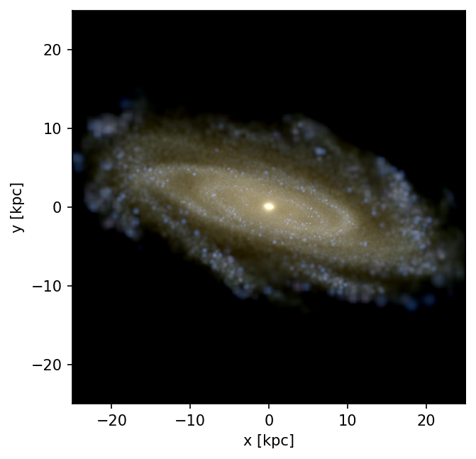
Stars#
There are a number of ways to visualize the stellar content of a simulation. One can of course pass the star particles to the same image functions as above, but there are also some more specialized functions. Here, we make an RGB image covering the magnitude range 18 to 26 \(\mathrm{mag/arcsec}^2\). This consults SSP models to estimate the luminosity of each star particle, and then projects these luminosities to make an image. The default bands are \(i\), \(v\) and \(b\), but
these can be changed with the r_band, g_band and b_band keyword arguments.
In [16]:
pynbody.plot.stars.render(f.st, width="50 kpc", mag_range=[18, 26])
/Users/app/Science/pynbody/pynbody/array/__init__.py:361: RuntimeWarning: invalid value encountered in log
  result = super().__array_ufunc__(ufunc, method, *inputs, **kwargs)
In reality, the galaxy would be obscured by the dust content in the gas. To estimate this effect, we can set with_dust=True. The dust model is exceptionally simple, so for detailed scientific analysis one should use a specialist radiative transfer package like Skirt. Nonetheless, it gives a reasonable first estimate of the dust effects.
In [17]:
pynbody.plot.stars.render(f, width="50 kpc", with_dust=True, mag_range=[18, 26])
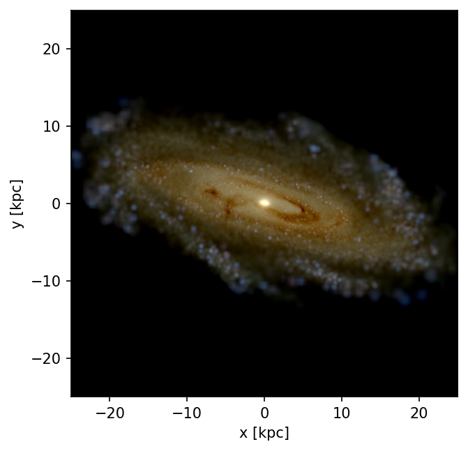
Dust is estimated simply by assuming that the dust-to-metals ratio is constant. This results in dust
correlated with high density, high metallicity regions. For more information see the reference documentation
for pynbody.plot.stars.render().
The resulting correlation of the dust with spiral arms and star formation regions is clearer when rendered face-on:
In [18]:
with pynbody.analysis.faceon(h[0]):
    pynbody.plot.stars.render(f, width="50 kpc", with_dust=True, mag_range=[18, 26])

Another specialised routine is pynbody.plot.stars.contour_surface_brightness, which can be used to overlay contours of surface brightness
on top of an existing image. For example, if we are interested in the line-of-sight velocity structure of a galaxy,
we can produce a v-band luminosity-density weighted velocity image. Note that the luminosity density can be automatically
derived by accessing the v_lum_den array; see the reference documentation for pynbody.analysis.luminosity.
We can plot the actual contours of v-band surface brightness over the top using contour_surface_brightness().
We pass in a smooth_min keyword argument to smooth the contours appropriately.
In [19]:
pynbody.plot.sph.image(f.st, qty='vz', cmap='PuOr', width='50 kpc', weight='V_lum_den',
                       log=False, vmin=-200, vmax=200)
pynbody.plot.stars.contour_surface_brightness(f.st, 'V', width="50 kpc",
                                               contour_kwargs={'colors': 'black',
                                                               'levels': [22, 24, 26, 28]},
                                               smooth_floor='1.0 kpc')

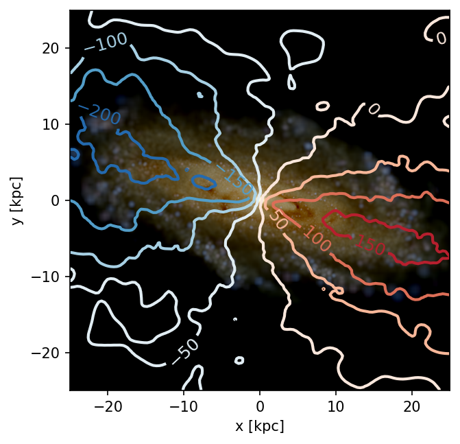
A more general version of the contouring routine is pynbody.plot.sph.contour, which can be used to overlay contours of any quantity. Here we swap the emphasis of the previous figure, plotting contours of the luminosity-weighted average line-of-sight velocity over an image of the stellar emission.
In [20]:
pynbody.plot.stars.render(f, width="50 kpc", with_dust=True, mag_range=[18, 26])
pynbody.plot.sph.contour(f.stars, 'vz', weight='V_lum_den', smooth_floor='0.5 kpc', width="50 kpc",
                         contour_kwargs={'cmap': 'RdBu_r', 'linewidths': 2}, log=False)
Spherical images#
Pynbody can also render images to healpix format, providing an all-sky image as seen from the current origin.
Note
Pynbody does not require healpy installed to produce the map, but if you want to visualise the map then you do need healpy installed to perform the 2D Mollweide projection.
Use pip install healpy to obtain healpy.
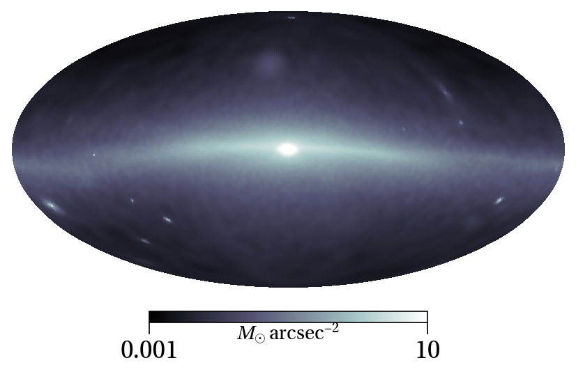
The function pynbody.plot.sph.spherical_image() operates very similarly to
image(), so getting a basic mass map is easy. As an example, let’s
look at the view of the density of stars from a solar-like position in this galaxy:
In [21]:
with pynbody.analysis.faceon(h[0]).translate([8,0,0]):
    pynbody.plot.sph.spherical_image(h[0].st, 'rho', cmap='bone', units="Msol arcsec^-2",
                                     vmin=1e-3, vmax=10.)
In [22]:
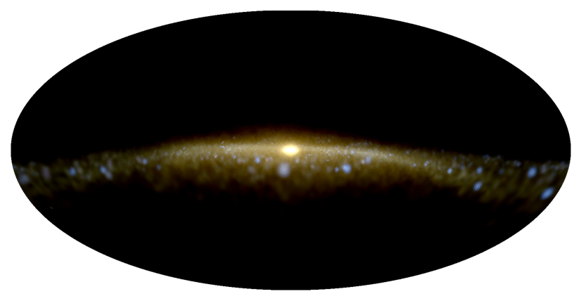
with pynbody.analysis.faceon(h[0]).translate([9.0,0,0]):
    pynbody.plot.stars.render_mollweide(h[0],  mag_range=(18,22))
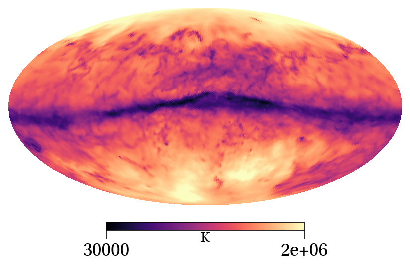
You can produce weighted plots too; for example here is the density-weighted temperature for the gas, from the same position:
In [23]:
with pynbody.analysis.faceon(h[0]).translate([8,0,0]):
    pynbody.plot.sph.spherical_image(h[0].gas, 'temp', weight='rho', cmap="magma",
                                    vmin=3e4, vmax=2e6)
See also
The pynbody imaging system is very flexible. To start understanding more about the options available, see the
reference documentation for pynbody.plot.sph.image(), pynbody.plot.sph.velocity_image(), pynbody.plot.stars.render(),
pynbody.plot.stars.contour_surface_brightness() and pynbody.plot.sph.contour().
In addition, pynbody has a companion package, topsy, which enables real-time rendering of snapshots on a GPU. See its separate website for more information.