Halos in Pynbody

Changed in version 2.0: Changes to the halo catalogue system, especially affecting AHF

If migrating from version 1.x, please see relevant warnings in the reference documentation.

Finding the groups of particles that encompass galaxies is the key first step of simulation analysis. Generally speaking, groups of particles that are gravitationally bound are known as ‘halos’, while unbound collections of particles are known simply as ‘groups’. Some literature also talks about ‘subhalos’, which are smaller groups of particles that are gravitationally bound within a larger halo. However, the nomenclature around groups, halos and subhalos is not consistent across the literature, and different halo finders may use different terminology. In pynbody, we use the term ‘halo’ to refer to any group of particles that has been identified by a finder and stored on disk. Thus, a pynbody Halo may represent a halo, a group, or a subhalo, depending on the context in which it was created.

There are several public group / halo finders available. Pynbody presents a common interface to these to the maximum extent possible. For a list of supported halo finders, see Supported halo-finder formats.

Note

The principal development of pynbody took place in the UK, and the spelling of “catalogue” is British English. However, since much code is written in American English, v2.0.0 introduced aliases such that all classes can be accessed with the American spelling HaloCatalog, AdaptaHOPCatalog etc.

To load a catalogue, call the halos() method on a loaded simulation snapshot. Pynbody scans the disk looking for files that follow the naming convention of known halo finders.

For example, with the pynbody test data, we can load halo catalogues as follows:

In [1]: import pynbody
   ...: import matplotlib.pylab as plt
   ...: 

In [2]: s = pynbody.load('testdata/gasoline_ahf/g15784.lr.01024.gz')

In [3]: s.halos()
Out[3]: <AHFCatalogue, length 1411>

In this case, we have loaded a simulation snapshot from the Gasoline code, for which an AHF halo catalogue is available. Pynbody has automatically detected the presence of the AHF catalogue and loaded it for us. Here is another example from the test data:

In [4]: s = pynbody.load('testdata/gadget4_subfind_HBT/snapshot_034.hdf5')

In [5]: s.halos()
Out[5]: <Gadget4SubfindHDFCatalogue, length 2517>

The Gadget4 snapshot has a SubFind halo catalogue, which pynbody has loaded for us. However, in this particular case there is _also_ and HBT+ catalogue available. To load this, we can specify the halo finder priority either in the configuration file (see Configuring pynbody) or at runtime.

Selecting a format

If you have more than one halo catalogue available, or if your halo catalogue is not in the default location, you need to provide additional information to the halos() method.

To specify a particular halo finder, use the priority keyword argument. For example, to load the HBT+ catalogue for the Gadget4 snapshot, we can do:

In [6]: s.halos(priority=['HBTPlusCatalogue'])
Out[6]: <HBTPlusCatalogue, length 2349>

Notice that pynbody has now loaded the HBT+ catalogue instead of the SubFind catalogue.

Note

In the specific case of HBT+, halos are found within the parent groups of a SubFind catalogue. To see the full hierarchy of structure in this snapshot requires using both catalogues together. More information about this is given in the reference documentation.

For a list of the available halo finders, see Supported halo-finder formats. You can either pass classes or strings naming them to the priority argument.

As described in Configuring pynbody, you can also tell pynbody which group finders you prefer in your configuration file. The priority argument is used to override this default preference at runtime.

Specifying locations

If your halo catalogue is not in the default location, it probably will not be found automatically when you call the pynbody.snapshot.simsnap.SimSnap.halos() method. You can therefore specify the path to the catalogue using the filename keyword argument. This also functions as an alternative way to disambiguate between multiple halo catalogues. For example:

In [7]: s.halos(filename='testdata/gadget4_subfind_HBT/034/SubSnap_034.0.hdf5')
Out[7]: <HBTPlusCatalogue, length 2349>

In [8]: h = s.halos(filename='testdata/gadget4_subfind_HBT/fof_subhalo_tab_034.hdf5')

In [9]: h
Out[9]: <Gadget4SubfindHDFCatalogue, length 2517>

Note

Some halo finders produce multiple files, so the filename keyword argument is necessarily interpreted slightly differently by some readers. As a general guideline, if the halo finder output is of the form path/to/file.extension, path/to/file.another_extension etc, then the filename``argument should be the path to the basename (i.e.``path/to/file). For specific help, consult the reference documentation for the specific halo finder’s __init__; a list of these is available in Supported halo-finder formats.

Information about the catalogue

We will continue to use the Gadget4/SubFind sample catalogue for the following examples, and we assigned this to the variable h above.

We can easily retrieve some basic information, like the total number of halos in this catalogue:

In [10]: len(h)
Out[10]: 2517

To access the particle members of a halo, use square bracket syntax. For example, the following returns the number of particles in the first two halos, use

In [11]: len(h[0]), len(h[1])
Out[11]: (307386, 137037)

Note

Halo numbers to use are assigned by the halo finder, unless overriden by the user. Here, the first halo is halo 0, but that need not have been the case.

As may now be evident, the syntax for dealing with particles within an individual halo precisely mirrors the syntax for dealing with an entire simulation. For example, we can get the total mass in the first halo and see the position of its first few particles as follows:

In [12]: h[0]['mass'].sum().in_units('1e12 Msol')
Out[12]: SimArray(0.58234838, '1.00e+12 Msol')

In [13]: h[0]['pos'][:5]
Out[13]: 
SimArray([[23.750328, 27.66374 , 25.721956],
          [23.751205, 27.66415 , 25.72195 ],
          [23.75042 , 27.66385 , 25.722666],
          [23.75083 , 27.663345, 25.722668],
          [23.750278, 27.663668, 25.722883]], dtype=float32, '3.09e+24 cm a h**-1')

We might also be interested in the properties that a halo finder has calculated for each halo. For example, SubFind calculates various masses and names them GroupMass. This is accessible in the following way:

In [14]: h[0].properties['GroupMass']
Out[14]: Unit("7.80e+44 g h**-1")

Here, the units are currently not very user-friendly. Just as with a simulation snapshot, we can convert the units in a halo catalogue to something more useful:

In [15]: h.physical_units()

In [16]: h[0].properties['GroupMass']
Out[16]: Unit("5.82e+11 Msol")

Calling physical_units() on a halo catalogue object will convert all properties, and additionally all particle data, to the default pynbody units or a different set of units if specified. The call signature is the same as for SimSnap.physical_units.

For halo finders such as SubFind that support a hierarchical view of the structure, a subhalos attribute is provided:

In [17]: subhalos_of_0 = h[0].subhalos

In [18]: subhalos_of_0
Out[18]: <SubhaloCatalogue, length 135>

The subhalos_of_0 object behaves just like a regular catalogue, but it only contains the specified subhalos. So, for example, we can see the number of particles in the first subhalo, and its mass:

In [19]: len(subhalos_of_0[0]), subhalos_of_0[0].properties['SubhaloMass']
Out[19]: (215716, Unit("4.09e+11 Msol"))

Note

SubFind-specific information

SubFind distinguishes sharply between parent halos (known as FOF groups) and subhalos. Even the properties are different. For example, the mass of a subhalo is stored in the SubhaloMass property, while the mass of a parent halo is stored in the GroupMass property, as above.

The subhalos are not even available from the parent halo catalogue itself, i.e. running through all the halos in h will not give you the subhalos, in contrast to some other halo finders. If you want to be able to run through all subhalos within the entire simulation, you can load the subhalo catalogue directly using

all_subhalos = s.halos(subhalos=True)

Accessing particle data

When accessing halos in the above way, the particle data is also available. The object returned by h[0], h[1] etc is actually a Halo object, which is a subclass of SubSnap, which in turn is a subclass of SimSnap.

This means that you can access the particle data as though the halo were a simulation snapshot. For example, to get the particle masses of the first halo:

In [20]: h[0]['mass']
Out[20]: 
SimArray([1894518.1, 1894518.1, 1894518.1, ..., 1894518.1, 1894518.1,
          1894518.1], dtype=float32, 'Msol')

We can verify that this agrees with the halo-finder-calculated mass:

In [21]: h[0]['mass'].sum()
Out[21]: SimArray(5.8234864e+11, dtype=float32, 'Msol')

In [22]: h[0].properties['GroupMass']
Out[22]: Unit("5.82e+11 Msol")

The same is true for positions, velocities, etc. For example, to get the positions of the first 5 particles in the first halo:

In [23]: h[0]['pos'][:5]
Out[23]: 
SimArray([[16014.695, 18653.484, 17344.152],
          [16015.287, 18653.76 , 17344.148],
          [16014.757, 18653.559, 17344.63 ],
          [16015.033, 18653.219, 17344.63 ],
          [16014.662, 18653.436, 17344.777]], dtype=float32, 'kpc')

The same syntax can be used to access the particle data of subhalos. For example, to get the velocities of the first 5 particles in the first subhalo of the first halo:

In [24]: h[0].subhalos[0]['vel'][:5]
Out[24]: 
SimArray([[-76.89401 , 163.26326 ,  63.777664],
          [-83.55451 , 161.6504  ,  74.341225],
          [-87.5334  , 179.96936 ,  70.71324 ],
          [-94.90368 , 183.4485  ,  61.012352],
          [-69.53241 , 160.77155 ,  72.38382 ]], dtype=float32, 'km s**-1')

Working with large numbers of halos

Most halo finders will produce a large number of halos. Sometimes we are only interested in accessing a few, in which case the approaches above are sufficient. If, however, we access several in a row, pynbody may issue a warning unless one first calls load_all() to load all the halo data into memory. This is because pynbody is loading the data for each halo as it is accessed, and while this is efficient for a small number of halos, it can be slow if done repeatedly.

Once in memory, the data can be accessed without further warnings. For example, to calculate the velocity dispersion in each of a number of halos, we can do:

In [25]: h.load_all()

In [26]: h[0]['vel'].std() # for one
Out[26]: SimArray(148.29068, dtype=float32, 'km s**-1')

In [27]: v_std = [halo_i['vel'].std() for halo_i in h[:100]] # for the first 100

If we are interested in finder-calculated properties, there is an even faster way to access them without ever constructing individual halo particle data objects. For example, to get the masses of halos, we can do:

In [28]: h.get_properties_one_halo(0)['GroupMass'] # for one, without touching any particles
Out[28]: Unit("5.82e+11 Msol")

In [29]: masses = h.get_properties_all_halos()['GroupMass'][:100] # for first 100, without touching any particles

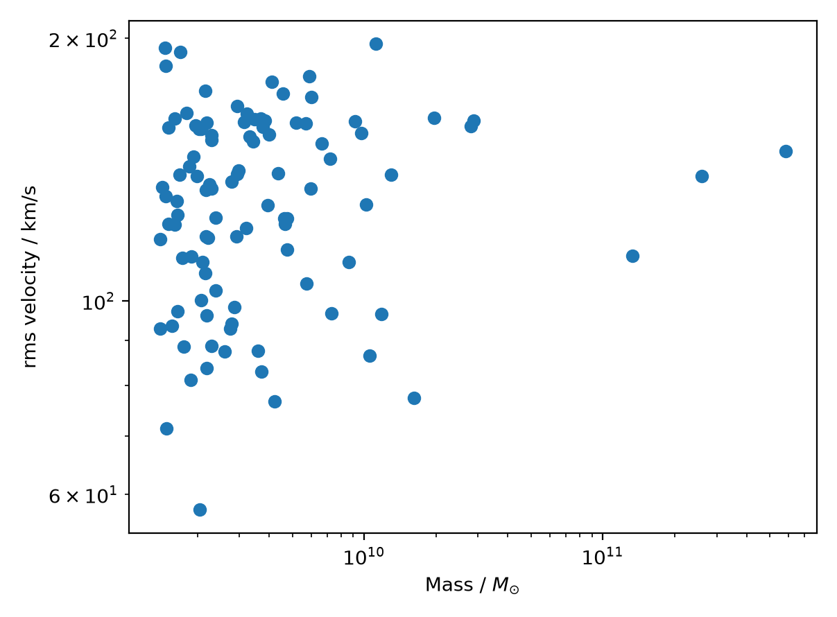
This is much faster than constructing individual halo objects, and is the recommended way to access finder-calculated properties when you are not interested in the particle data. We can now take a look at the velocity dispersion as a function of mass in this halo catalogue:

In [30]: plt.plot(masses, v_std, 'o')
Out[30]: [<matplotlib.lines.Line2D at 0x7f1993eb5050>]

In [31]: plt.xlabel(r'Mass / $M_{\odot}$')
Out[31]: Text(0.5, 0, 'Mass / $M_{\\odot}$')

In [32]: plt.ylabel(r'rms velocity / $\mathrm{km/s}$')
Out[32]: Text(0, 0.5, 'rms velocity / $\\mathrm{km/s}$')

In [33]: plt.loglog()
Out[33]: []

Note

Pynbody includes infrastructure for analysing large simulations and halo catalogues using parallel processing. This is used by its sister project, tangos, which offers a way to collate and analyse halo data across different timesteps and simulations, generating rich interactive databases which can then be queried and visualised in a variety of ways.